Multi-Modal Methods: The M Tank, 2018
Multi-Modal Methods:
Recent Intersections Between Computer Vision and Natural Language Processing
Edited for The M Tank by
Daniel R. Flynn*
Fernando Germán Torales Chorne*
Benjamin F. Duffy*
The M Tank
*Equal Contribution
Available on Medium: Part One, Part Two
Introduction
In this series of pieces we decided to examine the interplay between Computer Vision (CV) and Natural Language Processing (NLP) — a fitting segue from the previous CV-centric piece (available here). [1] While advancements within a singular field are often impressive, knowledge, by its very nature, is additive and combinatorial. These characteristics mean that improvements and breakthroughs in one field may catalyse further progress in other fields. Often two seemingly distinct bodies of knowledge coalesce to push our understanding, technologies and solutions into exciting and unforeseen areas.
In our previous work, we briefly attempted to outline Computer Vision’s claim on intelligence; building systems that can learn, infer and reason about the world from visual data alone. Here we hope to add to this discussion; what part does language play in the creation and recreation of intelligence?
This topic, when broached, has historically been a source of contention among linguists, neuroscientists, mathematicians and AI researchers. We can at least say that vision and language are inextricably intertwined, from an evolutionary standpoint, with the human experience. An experience that weighs learning heavily. For instance, when the concept of a ‘cat’ is evoked in your mind, there are numerous different associations around the nexus of cat almost instantly. Such as:
-
An image of a generic cat or a specific cat
-
The feeling of petting a cat’s soft fur
-
The letters ‘c’, ‘a’ and ‘t’
-
Sometimes-selfish and largely independent creatures
These basic experiences of the concept ‘cat’ all inform our understanding of what a cat is and its relationship to us and the world. This knowledge of ‘cat’ is iterable; it may be altered through direct experience, pondering cat-related things or by gaining information through any medium. Although not all experiences require language when recalling, the articulation of the experience or thought to oneself is often through language. If Computer Vision recognises patterns, then perhaps the addition of NLP could augment this process. It could enable processes in machines analogous to how people associate many modalities and experiences with the aforementioned concept of ‘cat’. The addition of language may eventually provide a means for machines to group, reason and articulate complex concepts in the future.
Much the same way we iterate, link and update concepts through whatever modality of input our brain takes — multi-modal approaches in deep learning are coming to the fore. Below are just some of the intersections between CV and NLP:
-
Lip Reading — Input is visual; output is text
-
Image Captioning — Input is visual; output is text
-
Visual Question Answering — Input is visual and text (question); output is text
-
Image Generation from Captions — Input is text; output is visual
Of these fields, we hope to provide insight into the progression and techniques of Lip Reading and Image Captioning in this series. While Visual Question Answering and Image Generation from Captions may be the subject of some future work.
In Deep Learning: Practice and Trends (NIPS 2017), [2] prominent researchers offered a simple abstraction — that virtually all deep learning approaches can be characterised as either augmenting architectures or loss functions, or applying the previous to new input/output combinations. While an oversimplification, the generalisability of current deep learning approaches is impressive. And as we shall see, these general approaches are also circumscribing new territories of competence as they progress.
There are also interesting second-order effects due to the generalisability of these methods and their relatively recent successes across-domains. This is despite the seemingly-troublesome issue of handling completely different inputs and output formats. Researchers can now work in many different areas and apply their techniques to issues across the spectrum, from social sciences to healthcare, and from sports to finance. Regardless of application, the tricks and knowledge gathered on architectures and loss functions may be repurposed and used anew somewhere else.
This partial disintegration of some research silos, or the encouragement of greater interdisciplinary work using AI-tools and techniques, follows on from our remarks about the combinatorial nature of knowledge. Second-order effects mean that CV researchers often understand NLP techniques, and vice-versa. Introductory courses and books on deep learning cover use cases within NLP, CV, Reinforcement Learning and Generative models.
In some senses, we are getting closer to a generalisable artificial intelligence; knowledge in deep learning is consolidating into a more paradigmatic approach. Such congruency allows researchers from all disciplines to leverage AI in new and exciting ways. Perhaps, a true general intelligence lies ahead, although how many paradigms must be disequilibrated and reinstated anew before such a point is reached is unknown. What we do know is that work in generalisable models continues to captivate us, as we watch techniques perform across multiple tasks, domains and modalities. [3][4][5]
In keeping with the last publication, we aim to be as accessible as possible for our audience, and to provide individuals with the tools to learn about AI at whatever depth they desire. However, in this piece we sacrificed expanse for greater depth into the research areas themselves. We will continue to experiment with scope and timelines, to understand how best to convey topics to the reader. For those lacking technical proficiency there may be short sections which are tedious; but their omission won’t impinge the lay-reader greatly. We hope that one should be able to take something of value away regardless of their skillset.
Further inroads will be made in the coming years into a greater number of fields, with better techniques deployed at an ever-increasing rate. Understanding that our assumptions may be incorrect, about what AI can and can’t do, is an important step for society. Ultimately, these technologies aim to emulate and improve the processes through which we navigate the world around us. To learn their own meta-structures for the world that we deploy everyday, subconsciously.
If humanity has never accepted limitations to our abilities, why would we assume that mechanised intelligence will be inherently limited in some way? And with new, unforeseen breakthroughs, the assumption that anyone can predict the long-term future of technology is perhaps untenable at best. The best strategy may be to simply stay as informed as we can and actively engage with the advancements on the horizon.
With thanks,
The M Tank Team![]()
Part One: Visual Speech Recognition (Lip Reading)
Previous work from the team detailed some of the many advancements within the field of Computer Vision. In practice, research isn’t siloed into isolated fields and, with this in mind, we present a short exploration of an intersection between Computer Vision (CV) and Natural Language Processing (NLP) — namely, Visual Speech Recognition, also more commonly known as lip reading.
Similar to the advancements seen in Computer Vision, NLP as a field has seen a comparable influx and adoption of deep learning techniques, especially with the development of techniques such as Word Embeddings [6] and Recurrent Neural Networks (RNNs). [7] Moreover, the drive to tackle complex, cross-domain problems using a combination of inputs has spawned much to be excited about. One source of excitement for us comes from seeing the skill of Lip Reading move from human-dominance to machine-dominance in the accuracy rankings. Another still from the method by which this was accomplished.
It was not so long ago that lip reading was heralded to be a difficult problem, much like the difficulty ascribed to the game of Go; albeit not quite as well-known. In addition to solving this problem, advancements in lip reading may potentially enable several new applications. For instance, dictating messages in a noisy environment, dealing with multiple simultaneous speakers better, and improving the performance of speech recognition systems in general. Conversely, extracting conversations from video alone may be an area of concern in the future.
Our focus on this niche application, one hopes, is both illustrative and informative. A relatively small body of deep learning work on lip reading was enough to upset the traditional primacy of the expertly-trained lip reader. Meanwhile, the combinatorial nature of AI research and the technologies at the centre of these advancements blend the demarcations between fields in a scintillating way. Where, if ever, such advancements plateau is the question on everyone's lips.
Framing the problem
The task of predicting innovations and advancements in technologies is notoriously quite difficult, and best reserved for small wagers between colleagues and friends. Where estimates are made, one usually compares a machine’s performance to tasks that humans are already good at, e.g. walking, writing, playing sports, etc. It surprised us to learn two things with regards to lip reading. Firstly, that machines managed to surpass expert-humans recently, and secondly, that expert-humans weren’t that accurate to begin with.
Irrespective of the bar set by the expert, we think it best to delve into what makes this a tough challenge to master. Visemes, analogous to the lip-movements that comprise a lip reading alphabet, pose a clear challenge to those who’ve ever attempted to apply them. Namely, that multiple sounds share the same shape. There exists a level of ambiguity between consonants, which cannot be dispensed with — a problem well documented by Fisher in his extensive study on visemes. [8]
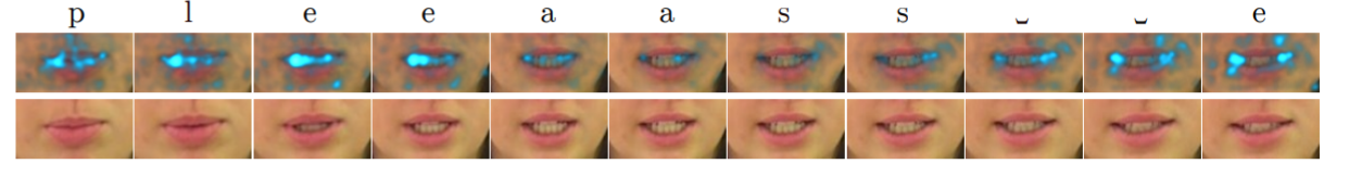
Figure 1: Viseme Examples
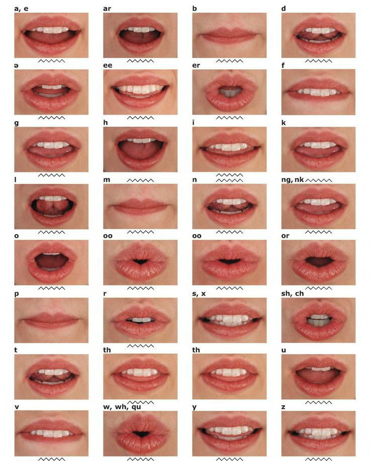
Note: This picture shows that several sounds, such as ‘p’ and ‘b’, have the same viseme, which means that the
corresponding phonemes are very difficult to determine for a person whose only information source is visual.
For example, saying the words “elephant juice” appears identical on the lips to “I love you”.
Source: Originally created by Dr Mary Allen and available from her site. [9]
Since there are only so many shapes that one’s mouth can make in articulation, mapping said shapes accurately to the underlying words is challenging. [10] Especially when much communication relies more on sound than on visual information; vocal communication is sound-dependent. Hence, achieving high accuracy without the context of the speech [11] is extremely difficult — for people and machines.
Early Results
With these limitations it’s not surprising that early studies focused on simplified versions of the problem. Initially, feature engineering produced improvements using facial recognition models which placed bounding boxes around the mouth, and extracted a model of the lips independent from the orientation of the face. Some common features used were the width-height ratio of a bounding box for detecting mouths, the appearance of the tongue (pixel intensity in the red channel of the image) and an approximation of the amount of teeth from the ‘whiteness’ in the image. [12]
Figure 2: Extracting Lips as a Feature
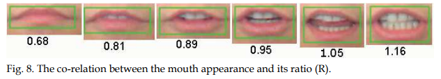
Note: The correlation between the mouth appearance and its ratio extracted independently from facial orientation.
Source: Hassanat (2011) [13]
These approaches obtained impressive results (over 70% word accuracy) for tests performed with classifiers trained on the same speaker they were tested on. But performance was heavily damaged when trying to lip read from individuals not included in the training set. Lip detection in males with moustaches was also more difficult and, therefore, the performance on such cases was poor. Hence, the feature engineering approaches, while an improvement, ultimately failed to generalise well.
Following this, using different viseme classification methods with defined language models improved state of the art (SOTA) performance. [14] Language models help filter results that are obviously incorrect and improve results by selecting from only plausible options, e.g. ‘n’ for the 4th character in "soon" rather than "soow" or "soog". Greater improvements still were made by "fine-tuning" the viseme classifier for phoneme classification, which enabled them to deal with multiple possible solutions for words containing the same visemes in similar intervals. This improved accuracy and performed comparatively better than previous approaches.
These early techniques brought performance to roughly 19% accuracy on an unseen test set, an improvement over the prior best of 17% (+/- 12%) accuracy generated by a sample of hearing-impaired lip readers. A sample group which outperforms the general population on average. [15]
McGurk and MacDonald argue in their 1976 paper [16] that speech is best understood as bimodal, that is taking both visual and audio inputs — and that comprehension in individuals may be compromised if either of these two domains are absent. Intuitively, many of us can recall mishearing speech while on the phone, or the difficulties one has in pairing sound and lips in a noisy environment. The requirement of bimodal inputs, as well as contextual constraints, hampers the ability of people and machines to read lips with accuracy. This pointed to the need for further studies on the use of these combined information sources. A direction which brings us into the most recent epoch of lip reading approaches.
The arrival of Deep Learning
It is with this point that we introduce recent work from Assael et al. (2016) — “LipNet: End-to-End Sentence-level Lipreading.” [17] “LipNet” introduces the first approach for an end-to-end lip reading algorithm at sentence level. Earlier work by Wand, Koutník and Schmidhuber [18] applied LSTMs [19] to the task, but only for word classifications. However, their earlier advances, including end-to-end [20] trainability, were undoubtedly valuable to the body of work in the space. For those wishing to know more about LSTMs and their variants, Christopher Olah provides an intuitive and detailed explanation of their use here. [21]
Figure 3: LipNet Example at Sentence Level
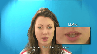
Note
: The speaker is saying “place blue”, and the “p” and “b” there have the same viseme, which means that the
corresponding phonemes are very difficult to accurately determine for a person whose only information source is
visual.
Source: GIF created by The M Tank, originally from
LipNet
video. [22]
On a high level in the architecture, the frames extracted from a video sequence are processed in small sets within a Convolutional Neural Network (CNN), [23] while an LSTM-variant runs on the CNN output sequentially to generate output characters. More precisely, a 10-frame sequence is grouped together in a block (width x height x 10), sequence length may vary, but the consecutive nature of these frames creates a Spatiotemporal CNN.
Then the output of this LSTM-variant, called a Gated Recurrent Unit (GRU), [24] is processed by a multi-layered perceptron (MLP) to output values for the different characters derived from the Spatiotemporal CNN. Lastly, a Connectionist Temporal Classification (CTC) provides final processing on the sequence outputs to make it more intelligible in terms of precise outputs, i.e. words and sentences. This approach allows information to be passed through the time periods comprising both words and, ultimately, sentences, improving the accuracy of network predictions.
The authors note that ‘LipNet addresses the issues of generalisation across speakers,’ i.e. the variance problems seen in earlier approaches, ‘and the extraction of motion features ’, originally classed as open problems in Zhou et al. (2014). [25] [26] The approach in LipNet, we feel, is interesting and exciting outside of the narrow confines of accuracy measures alone. The combination of CNNs and RNNs in the network — itself a hark back to our comments around the lego-like approach of deep learning research — is, perhaps, more evidence for the soon-to-be-primacy of differential programming. Deep Learning est en train de mourir. Vive Differentiable Programming! [27]
LipNet also makes use of an additional algorithm typically used in speech recognition systems — a Connectionist Temporal Classification (CTC) output. After the classification of framewise characters, which in combination with more characters define an output sequence, CTC can group the probabilities of several sequences (e.g. “c__aa_tt” and “ccaaaa__t”) into the same word candidates (in this case “cat”) for the final sentence prediction. Thus the algorithm is alignment-free. CTC solves the problem of matching sequences where timing is variable.
Figure 4: CTC in Action
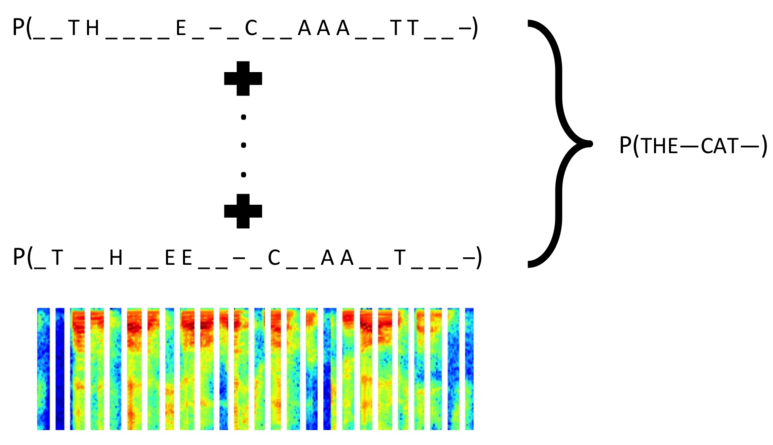
Note: CTC maps both representations shown in the image to the same sentence, “the cat”. This is despite differences in
spacing and elongation of letters/syllables. There is no need to find the perfect match or alignment between
framewise
output and classified character, the CTC loss function provides a unified, consistent output.
Source: Brueckner (2016) [28]
By predicting the alphabet characters and an additional “_” (space) character, it’s possible to generate a word prediction by removing repeated letters and empty spaces, as can be seen in fig. 5 for the classification of the word “please”. In practical terms this means that elongated pronunciations, variations in emphasis and timings, as well as pauses between syllables and words can still produce consistent predictions using the CTC for outputs.
Figure 5: Saliency map of “Please”
Note from source: Saliency shows the places where LipNet has learned to attend, i.e. the phonologically important regions. The
pictured transcription is given by greedy CTC decoding. CTC blanks are denoted by ‘⊔’.
Source: Assael et al. (2016, p. 7).
CTC is a function for output alignment and a loss correction function based on that alignment, and is independent of the CNN and LSTM-variants. One can also think of CTC as similar to a softmax due to converting the raw output of a network (e.g. raw class scores or in our case, characters) into the expected output (e.g. a probability distribution or in this case, words and sentences). CTC makes matching a single character output to word level possible. Awni Hannun provides an excellent dynamic publication that explains CTC operation; available here. [29]
There is a great video which covers some of LipNet’s functionality, as well as a specific use case — operating within autonomous vehicles. Seeing LipNet in operation ties together much of what we’ve discussed about the system so far. [30]
Architecture and results
A hallmark of this method is that the output labels are not conditioned on each other. For example, the letter ‘a’ in ‘cat’ is not conditioned on ‘c’ or ‘t’. Instead this relation is extracted by three spatio-temporal convolutions, followed by two GRUs which process a set number of the input images. The output from the GRUs then goes through a MLP to compute CTC loss (see fig. 6).
Figure 6: LipNet Architecture
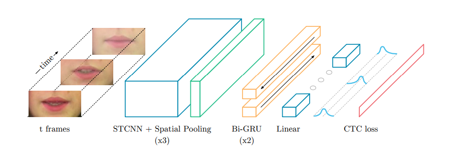
Note from source: LipNet architecture. A sequence of T frames is used as input, and is processed by 3 layers of STCNN, each followed
by a spatial max-pooling layer. The features extracted are processed by 2 Bi-GRUs; each time-step of the GRU output
is
processed by a linear layer and a softmax. This end-to-end model is trained with CTC.
Note: Bidirectional GRUs (Bi-GRUs) are an RNN variant that process the input in forward and reverse order.
Source: Assael et al. (2016, p. 5)
The architecture of LipNet was deemed an empirical success, achieving a prediction accuracy of 95.2% on sentences from the GRID dataset, an audiovisual sentence corpus for research purposes. [31] However, literature on deep speech recognition (Amodei et al., 2015) [32] suggested that further performance improvements would inevitably be achieved with more data and larger models. Commentators, reminded of earlier difficulties in generalisability and moustache-handling, expressed concern over the unusual sentences taken from GRID which formed the LipNet example video. The limited nature of GRID produced fears of overfitting; but how would LipNet fare in the real-world?
Figure 7: LipNet and other approaches
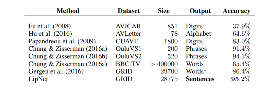
Note from source: Existing lipreading datasets and the state-of-the-art accuracy reported on these.
Source: Assael et al. (2016, p. 3)
The arrival of richer data
Not long after LipNet, DeepMind released ‘Lip Reading Sentences in the Wild’, [33] and addressed some of the concerns around LipNet’s generalisability. Taking inspiration from both CNNs for visual feature extraction [34] and the use of LSTMs for speech transcription, [35] the authors present an innovative approach to the problem of lip reading. By adding individual attention mechanisms for each of the input types, and combining them afterwards to produce character outputs, improvements in both the accuracy and generalisability of the original LipNet architecture were realised.
Attention mechanisms, discussed at length in part two of this piece, refer to a technique for focusing on specific parts of the input or previous layer(s) within neural networks. A somewhat-recent technique, taking inspiration from earlier work but popularised by Alex Graves’s in 2013/2014, it has grown in use partially from his memory-related work: the now-famous sequence generation paper [36] along with his work on neural turing machines. [37]
Attention mechanisms have been an enabler of some the recent success within deep learning; due to more efficient and clever processing of data. It also allows these models to have more interpretability, i.e. if asking why a network thinks a certain image is a dog it is often hard to look at and understand the internals of the network to find out why. Attention allows the network to highlight the salient parts of the image used in its prediction, e.g. a snout and pointed ears. Attention has become such a common technique that it spawned papers like “attention is all you need”, which foregoes convolution and recurrence techniques entirely for the problem of machine translation.
Returning to “Lip Reading Sentences in the Wild”, Chung et al. (2017) present their WLAS Network. Composed of three main submodules (watch, listen spell) — with attention sprinkled into the spell module. The system is as follows:
-
Watch (image encoder): Takes images and encodes them into a deep representation to be processed by further modules.
-
Listen (audio encoder): Allows the system to take in audio format as optional help to lip reading. This directly processes 13-dimensional MFCC features (see next section).
-
Spell (character decoder): This module incorporates the information from all previous modules. Each encoder above transforms their respective input sequence into a fixed-dimensional state vector and sequences of encoder outputs. The character decoder, which is a LSTM transducer, then reads the fixed state and attention vectors from both encoders and produces a probability distribution over the output character sequence. Finally, the attention vectors are fused with the output states to produce the context vectors that contain the information required to produce the next step output.
- Attend (independent regulation of audio and video attention mechanisms): Attend to what is important in each specific input signal/stream, i.e. audio or video. Without attention the model gets word error rates of over 100% and seems to forget the input signal. This shows that the dual-attention mechanism truly allowed this technique to work end-to-end. It also allows the network to handle out of sync audio/video (different sampling rates), including an absent stream.
WLAS functionality; greater details from more data
Watch is a VGG-M [38] that extracts a framewise feature representation to be consumed by an LSTM, which generates a state vector and an output signal. The Watch module looks at each frame in the video and extracts the relevant features that the module has learned to look for, i.e. certain lip movements/positions. This is done by a regular VGG-M CNN which outputs a feature representation for each frame.
This sequence of feature representations are then fed into a regular LSTM which generates a state vector (or cell state) and an output signal. With LSTMs and GRUs there’s an output and a “state” input to the next LSTM cell. The output is a character prediction (or a probability distribution of predicted character), while state is what encodes “the past”, i.e. what an LSTM has computed/stored of the past which is used to predict the next output.
Figure 8: Watch, Listen, Attend and Spell architecture
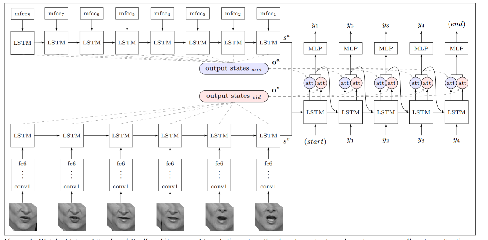
Note from source: “Figure 1. Watch, Listen, Attend and Spell architecture (WLAS). At each time step, the decoder outputs a character
yi, as well as two attention vectors. The attention vectors are used to select the appropriate period of the input visual and audio sequences.”
Source: Chung et al. (2017, p. 3)
The Listen module uses the Mel-frequency cepstral coefficients (MFCCs) [39] as its input. These parameters define a representation of the short-term power spectrum of a sound based on signal transformations. MFCCs ensure transformations are scaled to a frequency which simulates the human hearing range. Following this, independent attention mechanisms in the Attend module for each of the audio and video inputs are combined. These are then in turn passed through the Spell module. With a multi-layered perceptron (MLP) at each time step, the output from the LSTM ends up in a softmax to define the probabilities of the output characters.
With this, we return to similar themes of progress alluded to in our previous work: data availability and network stack-ability. Neural network-based approaches are typically characterised by heavy data demands. Concomitant to the progress in lip reading is the creation of a unique dataset for training and testing the network. Previously, research in lip reading was hampered by the available datasets and their small vocabularies. One only has to look at the desirable characteristics of Chung et al.’s (2016/2017) datasets, the LRW and the LRS, as expressed by Stafylakis and Tzimiropoulos (2017, p. 2), to understand the value of such data in improving research efforts:
“We chose to experiment with the LRW database, since it combines many attractive characteristics, such as large size (∼500K clips), high variability in speakers, pose and illumination, non-laboratory in-the-wild conditions, and target-words as part of whole utterances rather than isolated.” [40]
Chung et al. (2017) created a pipeline to automatically generate the dataset(s) [41] from BBC recordings as well as from the contained closed captions, which enabled progress in a data-intensive research area. Their creation is a ‘Lip Reading Sentences’ (LRS) dataset for visual speech recognition, consisting of over 100,000 natural sentences from British television.’
Figure 9: Pipeline to generate LRW/LRS dataset
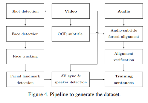
Steps: (A) Video preparation: (1) shot boundaries are detected by comparing colour histograms across consecutive frames.
(2) Face detection and grouping of the same face across frames. (3) Facial landmark detection. (4). (B) Audio and
text
preparation: (1) The subtitles in BBC videos are not broadcast in sync with the audio. (2) Force-align them, filter
and fix. (3) AV sync and speaker detection. (4) Sentence extraction.
The videos are divided into individual sentences/phrases using the punctuations in the transcript, e.g. by
full-stops,
commas, question marks, etc.
Source: Chung et al. (2017, p. 5)
The authors also corrupt said datum with storm noises (i.e. weather storms [42], demonstrating the network’s ability to use distorted and low volume data, or to discard audio completely for prediction purposes. Determining whether there’s value to the prediction in listening or not. For those wishing to see more, Joon Son Chung presents a fantastic overview of the authors’ work at CVPR. [43]
Although movements towards lower data requirements are pressing-on, this paradigm has yet to shift; and it’s likely that it shall remain this way for some time to come. As for stackability, the very nature of the LipNet and Lip Reading in the Wild architectures illustrate the lego-like nature of neural nets — e.g. CNNs plugged into RNNs with attention techniques. [44] While it’s true that this is a gross oversimplification, as a heuristic we find it increasingly useful in interpreting and understanding the rapid advancements across a lot of existing, and new, AI research.
Here this last point extends outside of the architecture itself, inscribing the potential stacking of inputs into our heuristic also. A great contribution of these works is the creation of an end-to-end architecture capable of using audio, video, or combinations of both as inputs to generate a text prediction as output: creating a truly multimodal model. Multiple input sequences resulting in a singular output sequence. Solving this multi-modal problem, and others like it, potentially opens new paths to explore in connecting video, audio and language systems.
New paths of exploration
Curious as to what would follow the approaches detailed previously, we turn our attention to some of the most recent work in this space. Although not exhaustive, here’s a smattering of the best improvements we came across in this domain:
-
Combining Residual Networks with LSTMs for Lipreading: [45] Improves on the original LRW paper by using a spatiotemporal convolutional network, a residual network and stacked bidirectional Long Short-Term Memory networks (BiLSTMs). The latter of which processes the input features in forward and reverse order like the BiGRU mentioned earlier. Their approach improves from 76.2% to 83% word accuracy [46] on the LRW paper, and also improves the accuracy on the GRID dataset. They do not extend, at present, to sentences on the LRS dataset.
-
Improving Speaker-Independent Lipreading with Domain-Adversarial Training:[47] Helps improve the performance on a target speaker with only a small amount of data. It isn’t as effective in instances where the model is trained on a lot of data. Hence, we would be interested to see its performance on LRS which has a 1000+ speakers.
-
End-to-End Multi-View Lipreading: [48] Achieves classification of non-frontal lip views, also utilising Bidirectional Long-Short Memory (BiLSTM). For each viewpoint the authors create an identical encoding MLP architecture (a stream of video processing), which enables the network to train with multiple views simultaneously (see fig. 10).
Figure 10: Architecture
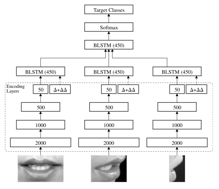
Note from source: Overview of the end-to-end visual speech recognition system. One stream per view is used for feature extraction
directly from the raw images. Each stream consists of an encoder which compresses the high dimensional input image
to
a low dimensional representation. The ∆ and ∆∆ features are also computed and appended to the bottleneck layer. The
encoding layers in each stream are followed by a BiLSTM which models the temporal dynamics. A BiLSTM is used to fuse
the information from all streams and provides a label for each input frame.
Note: ∆ and ∆∆ refer to the first and second derivatives from the encoded feature maps right before each BiLSTM,
respectively. Using these representations forces the encoding MLPs to create encoded features with meaningful
information on its derivatives as opposed to the use of derivatives on the image level. [49]
Source
: Petridis et al. (2017, p. 3)
-
Visual Speech Enhancement using Noise-Invariant Training: [50]
Tackles a somewhat related problem by providing a method for enhancing the voice of visible speakers in noisy
environments. The approach uses the audio-visual inputs seen previously to disentangle the voice from background
noise by matching lip movements. Although it differs from the other approaches, the idea itself is novel and,
frankly, pretty cool. Especially since it makes use of a lipreading dataset for this task.
“Visual speech enhancement is used on videos shot in noisy environments to enhance the voice of a visible speaker and to reduce background noise. While most existing methods use audio-only inputs, we propose an audio-visual neural network model for this purpose. The visible mouth movements are used to separate the speaker’s voice from the background sounds“
Update August 30th 2019: Two new papers from the authors of LipNet and Lip Reading in the Wild respectively.
- Large-Scale Visual Speech Recognition
- Deep Lip Reading: a comparison of models and an online application
Part Two: Image Captioning (From Translation to Attention)
Figure 11: Some image captioning examples
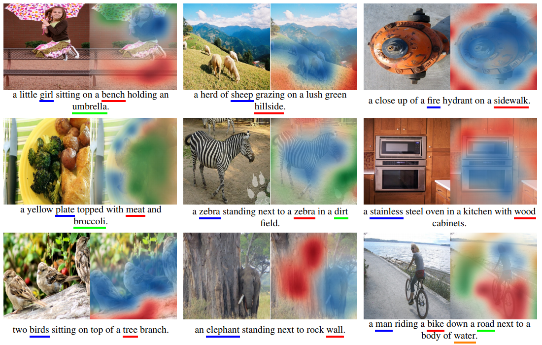
Note from source: Visualisation of generated captions and image attention maps on the COCO dataset. Different colors show a
correspondence between attended regions and underlined words, i.e. where the network focuses its attention in
generating the prediction.
Note: Cropped from the full image which provides more failure examples. For instance, the birds in the bottom left are
miscounted as two instead of three.
Source: Lu et al. (2017) [51]
Introduction to Image Captioning
Suppose that we asked you to caption an image; that is to describe the image using a sentence. This, when done by computers, is the goal of image captioning research. To train a network to accurately describe an input image by outputting a natural language sentence.
It goes without saying that the task of describing any image sits on a continuum of difficulty. Some images, such as a picture of a dog, an empty beach, or a bowl of fruit, may be on the easier end of the spectrum. While describing images of complex scenes which require specific contextual understanding — and to do this well, not just passably — proves to be a much greater captioning challenge. Providing contextual information to networks has long been both a sticking point, and a clear goal for researchers to strive for.
Image captioning is interesting to us because it concerns what we understand about perception with respect to machines. The problem setting requires both an understanding of what features (or pixel context) represent which objects, and the creation of a semantic construction “grounded” to those objects. When we speak of grounding we refer to our ability to abstract away from specifics, and instead understand what that object/scene represents on a common level. For example, we may speak to you about a dog, but all of us picture a different dog in our minds, and yet we can ground our conversation in what is common to a dog and progress forward. Establishing this grounding for machines is known as the language grounding problem.
These ideas also move in step with the explainability of results. If language grounding is achieved, then the network tells me how a decision was reached. In image captioning a network is not only required to classify objects, but instead to describe objects (including people and things) and their relations in a given image. Hence, as we shall see, attention mechanisms and reinforcement learning are at the forefront of the latest advances — and their success may one day reduce some of the decision-process opacity that harms other areas of artificial intelligence research.
We thought that the reader may benefit from a description of image captioning applications, of which there are several. Largely, image captioning may benefit the area of retrieval, by allowing us to sort and request pictorial or image-based content in new ways. There are also likely plenty of opportunities to improve quality of life for the visually-impaired with annotations, real-time or otherwise. However, we’re of the opinion that image captioning is far more than the sum of its immediate applications.
Mapping the space between images and language, in our estimation, may resonate with some deeper vein of progress. Which, once unearthed, could potentially lead to contextually-sophisticated machines. And, as we’ve noted before, providing contextual knowledge to machines may likely be the one of the key pillars that eventually support AI’s ability to understand and reason about the world like humans do.
Image captioning in a nutshell: To build networks capable of perceiving contextual subtleties in images, to relate observations to both the scene and the real world, and to output succinct and accurate image descriptions; all tasks that we as people can do almost effortlessly.
Image captioning (circa 2014)
Image captioning research has been around for a number of years, but the efficacy of techniques was limited, and they generally weren't robust enough to handle the real world. Largely due to the limits of heuristics or approximations for word-object relationships. [52][53][54] However, in 2014 a number of high-profile AI labs began to release new approaches leveraging deep learning to improve performance.
The first paper, to the best of our knowledge, to apply neural networks to the image captioning problem was Kiros et al. (2014a), [55] who proposed a multi-layer perceptron (MLP) that uses a group of word representation vectors biased by features from the image, meaning the image itself conditioned the linguistic output. The timeline of this, and other advancements from research labs was so condensed, that looking back it seems like a veritable explosion of interest. These new approaches generally;
Feed the image into a Convolutional Neural Network (CNN) for encoding, and run this encoding into a decoder Recurrent Neural Network (RNN) to generate an output sentence. The network backpropagates based on the error of the output sentence compared with the ground truth sentence calculated by a loss function like cross entropy/maximum likelihood. Finally, one can use a sentence similarity evaluation metric to evaluate the algorithm.
One such evaluation metric is the Bilingual Evaluation Understudy algorithm, or BLEU score. The BLEU score comes from work in machine translation, which is where image captioning takes much of its inspiration; as well as from image ranking/retrieval and action recognition. Understanding the basic BLEU score is quite intuitive. A set of high-quality human translations are obtained for a given piece of text, and the machine's translation is compared against these human baselines, section by section at an n-gram [56] level. Typically an output score of ‘1' matches perfectly with the human translations, and a ‘0' means that the output sentence is completely unrelated to the ground truth. The most representative evaluation metrics within Machine Translation and Image Captioning include: BLEU 1-4 (n-gram with n=1-4), CIDEr, [57] ROUGE_L, [58] METEOR. [59] These approaches are quite similar in that they measure syntactic similarities between two pieces of text, while each evaluation metric is designed to be correlated to some extent with human judgement.
In image captioning however, translations are replaced with image descriptions or captions. But BLEU scores are still calculated as output against human-annotated reference captions. Hence, network-generated captions are compared against a basket of human-written captions to evaluate performance.
In the past we've noted the huge effect of new datasets on research fields in AI. The arrival of the Common Objects in Context (COCO) [60] dataset in 2014 ushered in one such shift in image captioning. COCO enabled data-intensive deep neural networks to learn the mapping from images to sentences. And, given a comparatively large dataset of images with multiple human-label descriptions of said images, coupled with new, clever architectures capable of handling image input and language output; it now became possible to train deep neural networks for end-to-end image captioning via techniques like backpropagation.
Translation of images to descriptions
In machine translation it is quite common to use ‘sequence-to-sequence' models. [61] These models work by generating a representation through a RNN, based on an input sequence, and then feeding that output representation to a second RNN which generates another sequence. This mechanism has been particularly effective with chatbots, enabling them to process the representation of the input query and generate a coherent answer related to the input sequence (sentence).
Figure 12: Sequence-to-sequence model
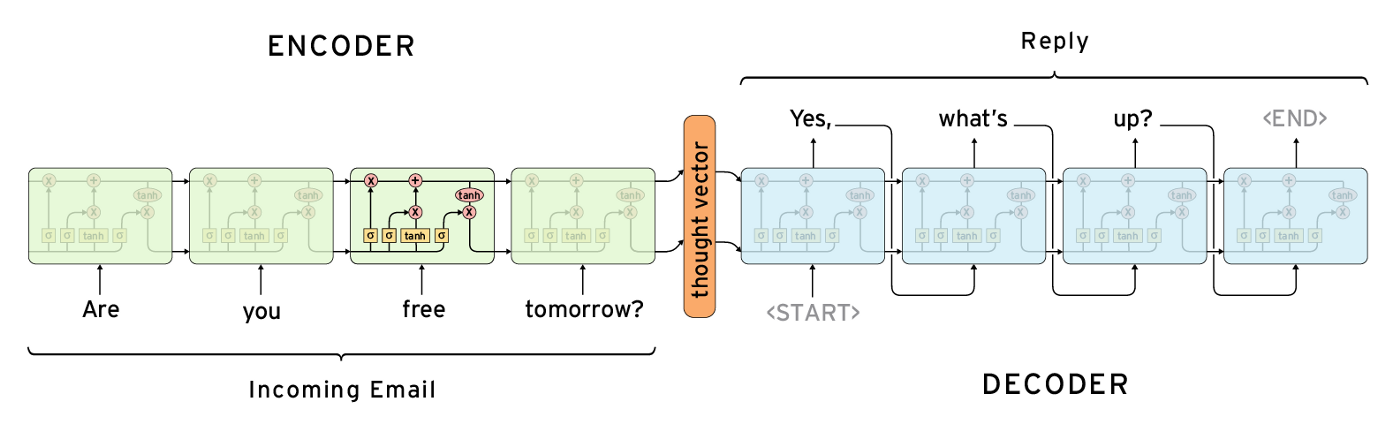
Note: This is an example of a sequence-to-sequence model used to generate automatic replies to messages. The same is
true for seq2seq models used for machine translation e.g. the right hand side could possibly output the translation
(in another language like Japanese) of the input words (left hand side). The encoder LSTM (in green) is “unrolled”
through time, i.e. every time step is represented as a different block that generates an encoded representation
(sometimes controversially known as a “thought vector”) as an output. After processing each word in the input
sentence, the final outputted encoding/hidden state can be used to set the initial parameters of the decoder LSTM
(in blue). The illustration shows how a word is generated at every time step. The complete set of generated words is
the output sequence (or sentence) of the network.
Source: Britz (2016) [62]
CNNs can encode abstract features from images. These can then be used for classification, object detection, segmentation, and a litany of other tasks. [63] Returning to the notion of contemporaneous successes in 2014, Vinyals et al. (2014) [64], successfully used a sequence-to-sequence model in which the typical encoder LSTM [65] was replaced by a CNN. In their paper titled, “Show and Tell: A Neural Image Caption Generator”, the CNN takes an input image and generates the feature representation which is then fed to the decoder LSTM for generating the output sentence (see fig. 13).
Figure 13: CNN encoder to LSTM decoder
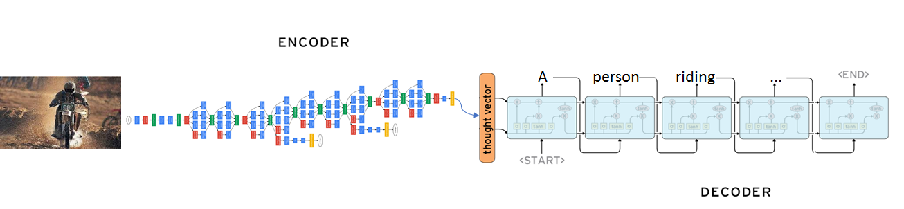
Note: The image is encoded into a context vector by a CNN which can then be passed to a RNN decoder. Different neural
blocks
of computation are combined in new ways to handle different tasks.
Source: The M Tank
A few more specifics on how the sentence is generated. At every step of the RNN, the probability distribution of the next word is outputted using a softmax. Depending on the situation, a slightly naive approach would be to take the word with the highest probability at each step after extracting the output from the RNN. However, beam search is another method which represents a better approach for sentence construction. By searching through specific combinations of words, and creating different possible outputs, beam search constructs a whole sentence without relying too heavily on any individual word from the ones which the RNN may generate at any specific time step. Beam search, therefore, can rank a lot of different sentences according to their collective, or holistic, probability.
Figure 14: Beam search example
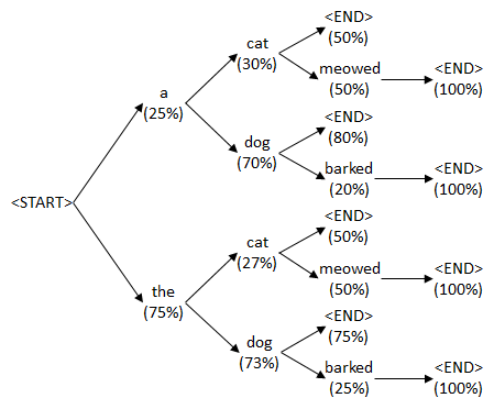
Source: Geeky is Awesome (2016) [66]
For example, at the first word prediction output step, a higher probability sentence might be outputted overall by choosing the word with a lower probability than the word with the highest. A deeper explanation of beam search for sentence generation, i.e. related to the decoder portion of our example above, may be found here. [67]
Further contemporaneous work
Around the time Show and Tell came around, a similar, but distinct, approach was presented by Donahue et al. (2014): Long-term Recurrent Convolutional Networks for Visual Recognition and Description. [68] Instead of just using an LSTM for encoding a vector, as is typically done in sequence-to-sequence models, the feature representation is outputted by a CNN, in this case VGGNet, [69] and presented to the decoder LSTM. This work was also successfully applied to video captioning, a natural extension of image captioning.
The main contribution of this work was not only this new connection setting between the CNN encoder and LSTM decoder, [70] but an extensive set of experiments which stacked LSTMs to try different connection patterns. The team also assess beam search against their own random sampling method, as well as using a CNN trained on ImageNet or further fine-tuning the pre-trained network to the specific dataset used. [71]
Delving deeper into the multimodal approach
From Captions to Visual Concepts and Back, by Fang et al. (2014), [72] is useful to explain multi-modality of the 2014 breakthroughs. Although distinct from the approaches of Vinyals et al. (2014) [73] and Donahue et al. (2014) [74], the paper represents an effective combination of some of these ideas. [75] For readers, the working flow of the captioning process may bring a new appreciation of the modularity of these approaches.
Figure 15: Creating captions from visual concepts
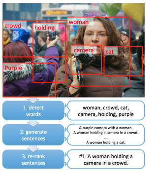
Source: Fang et al. (2014)
-
Detect words
To begin, it is possible to squeeze more information, which is easier to interpret, out of the CNN. Looking closer at how humans would complete the task, they would notice the important objects, parts and semantics of an image and relate them within the global context of the image. All before attempting to put words into a coherent sentence. Similarly, instead of “just” using the encoded vector representation of the image, we can achieve better results by combining information contained in several regions of the image.
Using a word detection CNN, which generates bounding boxes similar to what an object detection CNN does, the different regions in the image may receive scores for many individual objects, scenes or characteristics which correspond to words in a predefined dictionary (which includes about 1000 words).
-
Generate sentences
Next, the likelihood of the matched image descriptors (detections) are analysed according to a statistically predefined language model. E.g. if a region of the image is classified as “horse”, this information can be used as a prior to give a higher likelihood to the action of “running” over “talking” for the image captioning output. This combined with beam search produces a set of output sentences that are re-ranked with a Deep Multimodal Similarity Model (DMSM). [76]
-
Re-ranking sentences
This is where the multimodal independence comes into play. The DMSM uses two independent networks: a CNN for retrieving a vector representation of the image (VGG) and a CNN architecture with an explicit use. The image encoding network is based on the trained object detector from the previous section, with the addition of a set of fully connected layers to be trained for this re-ranking task. The second CNN is designed to extract a vector representation out of a given natural language sentence, which is the same size as the vector generated by the image encoding CNN. This effectively enables the mapping of language and images to the same feature space.
Since the image and encoded sentence are both represented as vectors with the same size, both networks are trained to minimise the cosine similarity between the image and ground truth captions for the given image, as well as to increase the difference with a set of irrelevant captions provided.
During the inference phase, the set of output sentences generated from the language model with beam search are re-ranked with the DMSM networks and compared against each other. The caption with highest cosine similarity is selected as the final prediction.
Dense captioning and the lead up to attention mechanisms (circa 2015)
Considerable improvements in bounding box detectors, such as RCNN, as well as the success of BiRNNs [77] in translation, produced another approach theoretically similar to the DMSM for sentence evaluation presented before. Namely, that one can make use of two independent networks, one for text and one for image regions, that create a representation within the same image-text space. An example of such an approach is seen in the work of Karpathy and Fei-Fei (2015). [78]
Deep Visual-Semantic Alignments for Generating Image Description [79] — which utilises the aforementioned CNN + RNN approach for caption generation — is, perhaps, most responsible for popularising image captioning in the media. A large proportion of articles on image captioning tend to borrow from their excellent captioned image examples.
But more impressive than capturing the public's attention with their research, were the strides made by Johnson, Karpathy and Fei-Fei later that year — in DenseCap: Fully Convolutional Localization Networks for Dense Captioning. [80]
Figure 16: Dense captioning & labelling
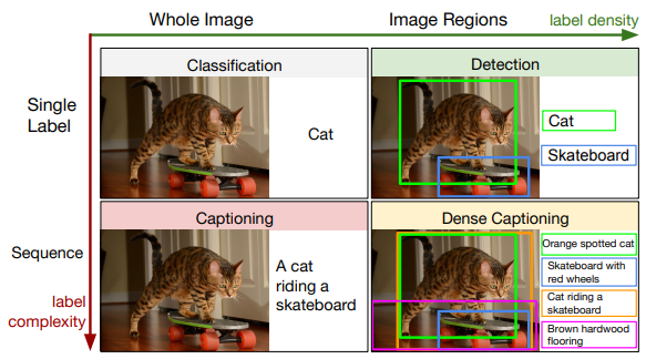
Note from source: We address the Dense Captioning task (bottom right) by generating dense, rich annotations with a single forward
pass.
Source: Johnson et al. (2015) [81]
We noted earlier that running a CNN into a RNN allowed the image features, and therefore, its information, to be output in natural language terms. Additionally, the improvements of RCNN inspired DenseCap to use a region proposal network to create an end-to-end model for captioning, with a forward computation time reduced from 50s to 0.2s using Faster-RCNN. [82]
With these technical improvements, Johnson et al. (2015) asked the question, why are we describing an image with a single caption, when we can use the diversity of the captions in each region of interest to generate multiple captions with better descriptions than an individual image caption provides?
The authors introduce a variation to the image captioning task called dense captioning where the model describes individual parts of the image (denoted by bounding boxes). This approach produces results that may be more relevant, and accurate, when contrasted with captioning an entire image with a single sentence. Put simply, the technique resembles object detection, but instead of outputting one word, it outputs a sentence for each bounding box in a given image. Their model also can be repurposed for image retrieval, e.g. “find me an image that has a cat riding a skateboard”. In this way we see the connection between image retrieval and image captioning is naturally quite common.
Figure 17: Dense captioning in action
Note from source: Example captions generated and localized by our model on test images. We render the top few most confident
predictions.
Source: Johnson et al. (2015)
We've seen improvements in information flow to the RNN, and the use of multiple bounding boxes and captions. However, if we placed ourselves in the position of captioner, how would we decide on the appropriate caption(s)? What would you ultimately deem important, or disregard, in captioning an image? What would you pay attention to?
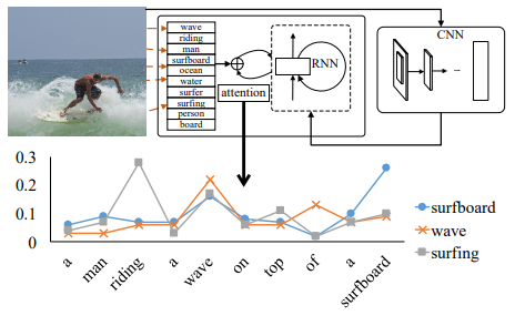
Enter “Show, Attend and Tell: Neural Image Caption Generation with Visual Attention” by Xu et al. (2015) [83] — the first paper, to our knowledge, that introduced the concept of attention into image captioning. The work takes inspiration from attention's application in other sequence and image recognition problems. Building on seminal work from Kiros et al. (2014a; 2014b), [84][85] which incorporated the first neural networks into image captioning approaches, the impressive research team of Xu et al. (2015) [86] implement hard and soft attention for the first time in image captioning.
Attention as a technique, in this context, refers to the ability to weight regions of the image differently. Broadly, it can be understood as a tool to direct the allocation of available processing resources towards the most informative parts of the input signal. Rather than summing up the image as a whole, with attention the network can add more weight to the ‘salient’ parts of the image. Additionally, for each outputted word the network can recompute its attention to focus on a different part of the image.
There are multiple ways to implement attention, but Xu et al. (2015) divide the image into a grid of regions after the CNN feature extraction, and produce one feature vector for each. These features are used in different ways for soft and hard attention:
-
In the soft attention variant, each region’s feature vector receives a weight (can be interpreted as the probability of focusing at that particular location) at every time step of the decoding RNN which signifies the relative importance of that region in order to generate the next word. The MLP (followed by a softmax), which is used to calculate these weights, is a deterministic part of the computational graph and therefore can be trained end-to-end as a part of the whole system using backpropagation as usual.
-
With hard attention only a single region is sampled from the feature vectors at every time step to generate the output word (using probabilities calculated similarly as mentioned before). This prevents the network training by backpropagation due to the stochasticity of sampling.
Training is instead completed using the final loss/reward (obtained from the sampled trajectory of chosen regions) as an approximation of the expected reward to be obtained from the MLP which, most importantly, can then be used to calculate the gradients. The same MLP is again used to calculate these probabilities [87]. The idea of sampling an attention trajectory as an estimation was taken from a Reinforcement Learning algorithm called REINFORCE [88]. The next part of this publication will deal with Reinforcement Learning applied to image captioning in different ways and with greater detail.
Figure 18: Attention in action
Note from source: Examples of attending to the correct object (white indicates the attended regions, underlines indicated the
corresponding word).
Source: Xu et al. 2015
Incorporating attention allows the decoder to focus on specific parts of the input representation for each of the outputted words. Meaning, that in converting aspects of the image to captions, the network can choose where and when to focus in relation to specific words outputted during sentence generation. Such techniques not only improve network performance, but also aid interpretability; we have a better understanding how the network determined its answer. As we shall see, attention mechanisms have grown in popularity since their inception.
Attention variants and interpretability
Attention and its variants come in many forms: Semantic attention, spatial attention and multi-layer attention. Hard, soft, bottom-up, top-down, spatial, adaptive, visual, text-guided, and so on. We feel that attention, while a newer technique for handling multi-modal problems, has the potential to be somewhat revolutionary.
Such techniques not only allow neural networks to tackle previously insurmountable problems, but also aid network interpretability; a key area of interest as AI permeates our societies. For those wishing to know more about attention, beyond the limited areas that we touch upon, there is an excellent distil article from Olah and Carter (2016) [89] available from here, and another by Denny Britz (2016) [90] available here.
Attention can enable our inspection and debugging of networks. It can provide functional insights, i.e. which parts of the image the network is ‘looking at’. Each form of attention, as we’ll see, has its own unique characteristics.
-
Image Captioning with Semantic Attention
(You et al., 2016) [91]
You et al. (2016) note that traditional approaches to image captioning are either ‘ top-down, moving from a gist of an image which is converted to words, or bottom-up, which generate words describing various aspects of an image and then combine them.’ [92] However, their contribution is the introduction of a novel algorithm that combines both of the aforementioned approaches, and learns to selectively attend. This is achieved through a model of semantic attention, which combines semantic concepts and the feature representation of the image/encoding.Semantic attention refers to the technique of focusing on semantically important concepts, i.e. objects or actions which are integral to constructing an accurate image caption. In spatial attention the focus is placed on regions of interest; but semantic attention relates attention to the keywords used in the caption as it’s generated.
There are several important differences, by the authors’ own admission, between their use of semantic attention and previous use-cases in image captioning. Comparing this work to Xu et al. (2015), [93] their attention algorithm learns to attend to the specific word concepts found within an image rather than words defined from specific spatial locations. It is important to note that some concepts or words may not be directly related to a specific region, e.g. the word “exciting” which may encompass the entire image. This is the case even with concepts that are not directly seen in the image, and can be expanded by ‘leveraging external image data for training additional visual concepts as well as external text data for learning semantics between words.’ [94]
Figure 19: Semantic attention framework
Note from source: Top — an overview of the proposed framework. Given an image, we use a convolutional neural network to extract a
top-down visual feature and at the same time detect visual concepts (regions, objects, attributes, etc.). We employ
a semantic attention model to combine the visual feature with visual concepts in a recurrent neural network that
generates the image caption.
Bottom — We show the changes of the attention weights for several candidate concepts with respect to the recurrent
neural network iterations.
Source: You et al. (2016) [95]
-
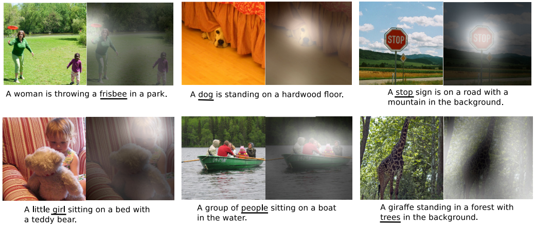
Next we introduce the concept of adaptive attention from Lu et al. (2017). [96]
Knowing When to Look: Adaptive Attention via A Visual Sentinel for Image Captioning
produced new benchmarks for state-of-the-art on both the COCO and Flickr30K datasets. Instead of forcing visual
attention to be active for each generated word, Lu et al. (2017) reason that certain words in a sentence do not
relate to the image, such as ‘the’, ‘of’, etc. Through the use of a
visual sentinel
the model learns
when
to use attention. Adaptive attention may also vary the amount of attention supplied for each word.
The Visual sentinel is classified as a latent representation of what the decoder already knows. As an extension of a spatial attention model, it determines whether the model must attend to predict the next word. We mentioned that words like ‘a’, ‘it’ and ‘of’ may be seen as not worth attending to; but words like ‘ball’, ‘man’ and ‘giraffe’ are not only worth attending at a point in time (sentinel), but also in a particular part of the image (spatial).
“At each time step, our model decides whether to attend to the image (and if so, to which regions) or to the visual sentinel. The model decides whether to attend to the image and where, in order to extract meaningful information for sequential word generation.” [97]
Figure 20: Visualisation of caption generation
Note from source: Visualization of generated captions, visual grounding probabilities of each generated word, and corresponding
spatial attention maps produced by our model.
Note: Knowing where and when, and how much to look. The probabilities graphed change depending on the ‘importance’ of
the word, i.e. the attention that should be given to an image section when generating the sentence.
Source: Lu et al. (2017) [98]
-
Another interesting piece is SCA-CNN: Spatial and Channel-wise Attention in Convolutional Networks for Image Captioning
from Chen et al. (2017). [99] The authors go all out
and make use of spatial, semantic, multilayer and multi-channel attention in their CNN architecture, while also
gently admonishing the use of traditional spatial attention mechanisms.
Attention is usually applied spatially to the final layer outputted by the encoder CNN, treating all channels the same to calculate where the attention should focus on, i.e. the usual attention model generates output sentences by only attending to specific spatial areas within the final convolutional layer.
“It is worth noting that each CNN filter performs as a pattern detector, and each channel of a feature map in CNN is a response activation of the corresponding convolutional filter. Therefore, applying an attention mechanism in channelwise manner can be viewed as a process of selecting semantic attributes.” [100]
‘CNN features are naturally spatial, channel-wise and multi-layer’ and the authors’ take full advantage of this natural design — applying attention to multiple layers within the CNN and to the individual channels within each layer.
Their approach was applied to the usual datasets of Flick8k, Flickr30k and COCO, and a thorough analysis of the different attention variants was undertaken. The authors note improvements in metrics both through combinations of attention variants, or with a single type, e.g. Spatial vs Channel vs Spatial + Channel. They also vary how many final layers the network should attend to (1-3), and extend this to different feature extractors, e.g. a VGG network (with attended layers being chosen from the “conv5_4, conv5_3 or conv5_2” convolution layers) or a ResNet.
The TencentVision team are leading the COCO captioning leaderboard at present. [101] According to the leaderboard, their entry description reads “multi-attention and RL”. When contrasted with the original paper, one must conclude that an approach which incorporates Reinforcement Learning techniques constitutes a variation on the original approach. However, we could not find a publication detailing these additions as of yet. [102]
-
In 2017,
Bottom-Up and Top-Down Attention for Image Captioning and Visual Question Answering
[103] from Anderson et al.
(2018) proposed a more natural method for attention, inspired by neuroscience. Another paper that truly explores
the difference between Bottom-Up and Top-Down attention, the authors’ examine attention in depth and present a
method to efficiently fuse information from both types.
“In the human visual system, attention can be focused volitionally by top-down signals determined by the current task (e.g., looking for something), and automatically by bottom-up signals associated with unexpected, novel or salient stimuli.” [104]Following from this definition, bottom-up attention is applied to a set of specific spatial locations which are generated by an object detection CNN. These salient spatial regions are typically defined by a grid on the image, but here they compute bottom-up attention over all bounding boxes where the detection network finds a region of interest. Specifically, each region of interest is weighted differently by a scaling/alpha factor and these are summed into a new vector which is passed into the language model LSTM. [105]
On the other hand, top-down attention uses an LSTM with visual information, [106] as well as task-specific context input, to generate its own weighted value of these features. The previously generated word, the hidden state from the language model LSTM and the image features averaged across all objects are used to generate the top-down attention output.
Using the same attention methodology, Anderson et al. (2018) managed to make strides in two different tasks, i.e. both image captioning and VQA. [107] Their approach is currently second on the COCO captioning leaderboard, [108] achieving SOTA scores on the MSCOCO test server with CIDEr / SPICE / BLEU-4 scores of 117.9, 21.5 and 36.9, respectively. [109]
“Demonstrating the broad applicability of the method, applying the same approach to VQA we obtain first place in the 2017 VQA Challenge”. [110]
Although attention and its variants represent quite a large body of impressive work, finally we turn ours, limited by space, to our last two favourite pieces of research to date:
-
MAT: A Multimodal Attentive Translator for Image Captioning
from Liu et al. (2017). [111] Liu et al. (2017) decide to pass the input image as a
sequence of detected objects to the RNN for sentence generation, as opposed to the favoured approach of having the
whole image encoded by a CNN into a fixed-size representation. They also introduce a sequential attention layer
which takes all encoded hidden states in to consideration when generating each word.
“To represent the image in a sequential way, we extract the object’s features in the image and arrange them in a order using convolutional neural networks. To further leverage the visual information from the encoded objects, a sequential attention layer is introduced to selectively attend to the objects that are related to generate corresponding words in the sentences.” [112]
-
Text-guided Attention Model for Image Captioning, from Mun et al. (2016), [113]
proposes a model which “combines visual attention with a guidance of associated text language
”, i.e. during training they use the training caption to help guide the model to attend to the correct things
visually. Their model can also use the top candidate sentences during testing to also guide attention. This method
seems to deal well with cluttered scenes.
“To the best of our knowledge, the proposed method is the first work for image captioning that combines visual attention with a guidance of associated text language.” [114]
![]()
References
[1] The M Tank. (2017). A Year in Computer Vision. [Online] TheMTank.com. Available: http://www.themtank.org/a-year-in-computer-vision
[2] Oriol Vinyals and Scott Reed (2017). Deep Learning: Practice and Trends (NIPS 2017 Tutorial, parts I & II). [Online Video] Steven Van Vaerenbergh (www.youtube.com). Available: https://www.youtube.com/watch?v=YJnddoa8sHk
[3] Kaiser et al. (2017). One Model To Learn Them All. [Online] arXiv: 1706.05137. Available: https://arxiv.org/abs/1706.05137v1
[4] Hashimoto et al. (2017). A Joint Many-Task Model: Growing a Neural Network for Multiple NLP Tasks. [Online] arXiv: 1611.01587. Available: arXiv:1611.01587v5
[5] Zamir et al. (2018). Taskonomy. [Website] Taskonomy/Stanford. Available: https://taskonomy.vision/
[6] Ruder, S. (2016). On word embeddings - Part 1. [Online] Sebastian Ruder Blog (ruder.io). Available: http://ruder.io/word-embeddings-1/
[7] Karpathy, A. (2015). The Unreasonable Effectiveness of Recurrent Neural Networks. [Online] Andrej Karpathy Blog (http://karpathy.github.io/). Available: http://karpathy.github.io/2015/05/21/rnn-effectiveness/
[8] Fisher, C.G. (1968). Confusions Among Visually Perceived Consonants. Journal of Speech, Language, and Hearing Research, December, Vol. 11, p. 796-804.
[10] Motion, pose (full-frontal view (0◦), angled view (45◦), and side view), Multiple people, video conditions/resolution/lighting, speech methods (accents, styles and rates of speech). Taken from: Bear, H.L. (2017, p. 25). Decoding visemes: Improving machine lip-reading. [Online] arXiv: 1710.01288. Available: arXiv:1710.01288v1. (Originally available 2016 from IEEE conference proceedings).
[11] Contexts of speech: subject, sound, time, place.
[12] Hassanat, A.B.A. (2011). Visual Speech Recognition. [Online] arXiv: 1409.1411. Available: arXiv:1409.1411v1.
[13] ibid
[14] Bear, H.L. (2017). Decoding visemes: Improving machine lip-reading. [Online] arXiv: 1710.01288. Available: arXiv:1710.01288v1. (Originally available 2016 from IEEE conference proceedings).
[15] Easton, R.D., Basala, M. (1982). Perceptual dominance during lipreading. Perception & Psychophysics, 32(6), p. 562-570.
[16] MacDonald, J., McGurk, H. (1976). Hearing Lips and Seeing Voices, Nature, volume 264, December, p. 746–748. Available: http://usd-apps.usd.edu/coglab/schieber/psyc707/pdf/McGurk1976.pdf
[17] Assael et al. (2016). Lipnet: End-to-End Sentence-Level Lipreading. [Online] arXiv: 1611.01599. Available: arXiv:1611.01599v2
[18] Wand et al. (2016). Lipreading with Long Short-Term Memory. [Online] arXiv: 1601.08188. Available: arXiv:1601.08188v1
[19] Long short-term memory (LSTM) is a type of unit within a Recurrent Neural Network (RNN) which is responsible for remembering and passing values over time periods. See: Hochreiter, S., Schmidhuber, J. (1997). Long Short Term Memory. Neural Computation, Vol. 9(8), p. 1735-1780. Available: http://www.bioinf.jku.at/publications/older/2604.pdf
[20] End-to-end, we define as, the joint training of all parameters within all parts of a neural network or system. In contrast to training them separately and in isolation.
[21] Olah, C. (2015). Understanding LSTM Networks. [Online] Colah’s Blog (http://colah.github.io/). Available: http://colah.github.io/posts/2015-08-Understanding-LSTMs/
[22] Assael, Y. (2016). LipNet: How easy do you think lipreading is? [Online Video] Yannis Assael www.youtube.com. Available: https://www.youtube.com/watch?v=fa5QGremQf8
[23] Karn, U. (2016). An Intuitive Explanation of Convolutional Neural Networks. [Online] Ujjwal Karn Blog (https://ujjwalkarn.me/author/ujwlkarn/). Available: https://ujjwalkarn.me/2016/08/11/intuitive-explanation-convnets/
[24] Cho et al. (2014). Learning Phrase Representations using RNN Encoder-Decoder for Statistical Machine Translation. [Online] arXiv: 1406.1078. Available: arXiv:1406.1078v3
[25] See Zhou et al. (2014). A review of recent advances in visual speech decoding. Image and Vision Computing, Vol. 32(9), p. 590–605.
[26] Quotes/reference taken from: Assael et al. (2016). Lipnet: End-to-End Sentence-Level Lipreading. [Online] arXiv: 1611.01599. Available: arXiv:1611.01599v2
[27] French comes courtesy of Google’s neural machine translation services. See Yann LeCun’s post: https://www.facebook.com/yann.lecun/posts/10155003011462143
[28] Brueckner, R. (2016). Accelerating Machine Learning with Open Source Warp-CTC. [Online] Inside HPC(insidehpc.com). Available: https://insidehpc.com/2016/01/warp-ctc/
[29] Hannun, A. (2017). Sequence Modeling With CTC. [Online] Distill (https://distill.pub/). Available: https://distill.pub/2017/ctc/
[30] Assael, Y. (2016). LipNet in Autonomous Vehicles | CES 2017. [Online Video] Yannis Assael (www.youtube.com). Available: https://www.youtube.com/watch?v=YTkqA189pzQ
[31] Barker et al. (2018). The GRID audiovisual sentence corpus. [Online] University of Sheffield. Available: http://spandh.dcs.shef.ac.uk/gridcorpus/ (last update, 18/03/2013).
[32] Amodei et al. (2015). Deep Speech 2: End-to-End Speech Recognition in English and Mandarin. [Online] arXiv: 1512.02595. Available: arXiv:1512.02595v1
[33] Chung et al. (2017). Lip Reading Sentences in the Wild. [Online] arXiv: 1611.05358. Available: arXiv:1611.05358v2
[34] Simonyan, K., Zisserman, A. (2015). Very Deep Convolutional Networks for Large-Scale Image Recognition. [Online] arXiv: 1409.1556. Available: arXiv:1409.1556v6
[35] Graves, A., Jaitly, N. (2014). Towards End-to-End Speech Recognition with Recurrent Neural Networks, Proceedings of the 31st International Conference on Machine Learning, Beijing, China, JMLR: W&CP volume 32. Available: http://proceedings.mlr.press/v32/graves14.pdf
[36] Graves, A. (2014). Generating Sequences With Recurrent Neural Networks. [Online] arXiv: 1308.0850. Available: arXiv:1308.0850v5
[37] Graves et al. (2014). Neural Turing Machines. [Online] arXiv: 1410.5401. Available: arXiv:1410.5401v2
[38] Chatfield et al. (2014). Return of the Devil in the Details: Delving Deep into Convolutional Nets. [Online] arXiv: 1405.3531. Available: arXiv:1405.3531v4
[39] Practical Cryptography. (2018). Mel Frequency Cepstral Coefficient (MFCC) tutorial. [Online] Practical Cryptography (http://www.practicalcryptography.com/). Available: http://www.practicalcryptography.com/miscellaneous/machine-learning/guide-mel-frequency-cepstral-coefficients-mfccs/ (accessed: 20/02/2018).
[40] Stafylakis, T., Tzimiropoulos, G. (2017). Combining Residual Networks with LSTMs for Lipreading. [Online] arXiv: 1703.04105v4. Available: arXiv:1703.04105v4
[41] Lip Reading Words (LRW) and Lip Reading Sentences (LRS)
[42] Multi-modal training. The audio stream is the easiest to learn from. During training they randomly select combinations of training with video, audio, or both. They also add noise to the audio to stop it from dominating the learning process, since Lip Reading is a much harder problem.
[43] Chung, J.S. (2017). Lip Reading Sentences in the Wild (Lip Reading Sentences Dataset), CVPR 2017. [Online Video] Preserve Knowledge (www.youtube.com). Available: https://www.youtube.com/watch?v=103CXDFhpcc
[44] Another trick this paper used was curriculum learning, which involves showing the network progressively more difficult data to learn during the training process. This can greatly speed up the training process and decrease overfitting. In this case, the model was first trained with single words, then 2-words, 3-words and, eventually, full sentences.
[45] Stafylakis, T., Tzimiropoulos, G. (2017). Combining Residual Networks with LSTMs for Lipreading. [Online] arXiv: 1703.04105v4. Available: arXiv:1703.04105v4
[46] Word Accuracy = 1 − Word error rate
[47] Wand, M., Schmidhuber, J. (2017). Improving Speaker-Independent Lipreading with Domain-Adversarial Training. [Online] arXiv: 1708.01565. Available: arXiv:1708.01565v1
[48] Petridis et al. (2017). End-to-End Multi-View Lipreading. [Online] arXiv: 1709.00443. Available: arXiv:1709.00443v1
[49] The idea behind it is that the derivatives of image features are associated with feature extractors (e.g. HoG, Sobel filter, etc.) https://www.learnopencv.com/histogram-of-oriented-gradients/
[50] Gabbay et al. (2017). Visual Speech Enhancement using Noise-Invariant Training. [Online] arXiv: 1711.08789. Available: arXiv:1711.08789v2
Part Two
[51] Lu et al. (2017). Knowing When to Look: Adaptive Attention via A Visual Sentinel for Image Captioning. [Online] arXiv: 1612.01887. Available: arXiv:1612.01887v2
[52] Kiros et al. (2014a): "Unlike many of the existing methods, our approach can generate sentence descriptions for images without the use of templates, structured prediction, and/or syntactic trees."
[53] Farhadi et al. (2010). Every Picture Tells a Story: Generating Sentences from Images. In: Daniilidis K., Maragos P., Paragios N. (eds) Computer Vision – ECCV 2010. ECCV 2010. Lecture Notes in Computer Science, vol 6314. Springer, Berlin, Heidelberg. Available: https://www.cs.cmu.edu/~afarhadi/papers/sentence.pdf
[54] Kulkarni et al. (2013). BabyTalk: Understanding and Generating Simple Image Descriptions. IEEE Transactions on Pattern Analysis and Machine Intelligence, Vol. 35, No. 12, December. Available: https://ieeexplore.ieee.org/stamp/stamp.jsp?arnumber=6522402
[55] Kiros et al. (2014a). Multimodal Neural Language Models. Proceedings of the 31st International Conference on Machine Learning, PMLR 32(2):595-603. Available: http://proceedings.mlr.press/v32/kiros14.html
[56] N-grams refer to the breakdown of a sequence of textual data into consecutive groups of symbols (e.g. words or letters). For example, in word bigrams (n=2), the sentence "A man riding a horse" breaks down to "A man", "man riding", "riding a", etc. These can then be used by specific evaluation metrics which give higher scores for output sentences that have more words in the same order as the ground truth.
[57] Vedantam et al. (2014). CIDEr: Consensus-based Image Description Evaluation. [Online] arXiv: 1411.5726. Available: arXiv:1411.5726v2 (2015 version).
[58] ROUGE stands for Recall-Oriented Understudy for Gisting Evaluation — Lin, C.Y. (2004). ROUGE: A Package for Automatic Evaluation of Summaries. Workshop on Text Summarization Branches Out, Post-Conference Workshop of ACL 2004, Barcelona, Spain. Available: http://www.aclweb.org/anthology/W04-1013
[59] Banerjee, S., Lavie, A. (2005). METEOR: An Automatic Metric for MT Evaluation with
Improved Correlation with Human Judgments. [Online] Language Technologies Institute, Carnegie Mellon University (www.cs.cmu.edu). Available: https://www.cs.cmu.edu/~alavie/papers/BanerjeeLavie2005-final.pdf
[60] Cocodataset.org. (2018) COCO: Common Objects in Context. [Website] http://cocodataset.org/. Available: http://cocodataset.org/#captions-challenge2015
[61] Sutskever et al. (2014). Sequence to Sequence Learning with Neural Networks. [Online] arXiv: 1409.3215. Available: arXiv:1409.3215v3
[62] Britz, D. (2016). Deep Learning for Chatbots, Part 1 – Introduction. [Blog] WildML (http://www.wildml.com/). Available: http://www.wildml.com/2016/04/deep-learning-for-chatbots-part-1-introduction/
[63] For shameless self-promotion, see previous report: “A Year in Computer Vision”. Available: http://www.themtank.org/a-year-in-computer-vision
[64] Vinyals et al. (2014). Show and Tell: A Neural Image Caption Generator. [Online] arXiv: 1411.4555. Available: arXiv:1411.4555v2
[65] LSTM (long-short term memory): a type of Recurrent Neural Network (RNN)
[66] Geeky is Awesome. (2016). Using beam search to generate the most probable sentence. [Blog] Geeky is Awesome (geekyisawesome.blogspot.ie). Available: https://geekyisawesome.blogspot.ie/2016/10/using-beam-search-to-generate-most.html
[67] ibid
[68] Donahue et al. (2014). Long-term Recurrent Convolutional Networks for Visual Recognition and Description. [Online] arXiv: 1411.4389. Available: arXiv:1411.4389v4 (2016 version)
[69] Visual Geometry Group Network (VGGNet), a type of neural network named after the research group who created it.
[70] This type of architecture was also tested by Vinyals et al. (2014) in their paper without success.
[71] Fine-tuning is a common practice which consists of training on a richer/larger dataset first (i.e. pretraining), and then retraining on the target dataset, since the generality of the features learned on the first dataset can often be used and transferred to some extent to the target dataset.
[72] Fang et al. (2014). From Captions to Visual Concepts and Back. [Online] arXiv: 1411.4952. Available: arXiv:1411.4952v3 (2015 version)
[73] Vinyals et al. (2014). Show and Tell: A Neural Image Caption Generator. [Online] arXiv: 1411.4555. Available: arXiv:1411.4555v2 (2015 version).
[74] Donahue et al. (2014). Long-term Recurrent Convolutional Networks for Visual Recognition and Description. [Online] arXiv: 1411.4389. Available: arXiv:1411.4389v4 (2016 version)
[75] Interestingly, although the authors hail primarily from Microsoft Research, contributions were made by researchers in Facebook AI Research (FAIR) and Google as well.
[76] Fang et al. (2014). From Captions to Visual Concepts and Back. [Online] arXiv: 1411.4952. Available: https://arxiv.org/abs/1411.4952v3 (2015 version).
[77] For more information see Part One: Visual Speech Recognition (Lip Reading). Medium: https://medium.com/mlreview/multi-modal-methods-part-one-49361832bc7e
[78] Karpathy, A., Fei-Fei, L. (2015). Deep Visual-Semantic Alignments for Generating Image Descriptions. [Online] Stanford Computer Science Department (cs.stanford.edu). Available: https://cs.stanford.edu/people/karpathy/cvpr2015.pdf. For additonal code, etc., see project page: https://cs.stanford.edu/people/karpathy/deepimagesent/
[79] ibid
[80] Johnson, J., Karpathy, A., Fei-Fei., L. (2015). DenseCap: Fully Convolutional Localization Networks for Dense Captioning. [Online] arXiv: 1511.07571. Available: arXiv:1511.07571v1
[81] ibid
[82] CNN computation only according to: Ren et al. (2015). Faster R-CNN: Towards Real-Time Object Detection with Region Proposal Networks. [Online] arXiv: 1506.01497. Available: arXiv:1506.01497v3 (2016 version).
[83] Xu et al. (2015). Show, Attend and Tell: Neural Image Caption Generation with Visual Attention. [Online] arXiv: 1502.03044. Available: arXiv:1502.03044v3 (2016 version)
[84] Kiros et al. (2014). Multimodal Neural Language Models. Proceedings of the 31st International Conference on Machine Learning, PMLR 32(2):595-603. Available: http://proceedings.mlr.press/v32/kiros14.html
[85] Kiros et al. (2014). Unifying Visual-Semantic Embeddings with Multimodal Neural Language Models. [Online] arXiv: 1411.2539. Available: arXiv:1411.2539v1
[86] The authors from Kiros et al. (2014) are present in the author list for Xu et al. (2015).
[87] A Multinoulli distribution is parameterised by the MLP and therefore, it can be sampled from. Using Monte-Carlo sampling, the final result from the sampling operation is that 1 region gets the entire weight and the rest get a weight of 0.
[88] Williams, R. J. (1992). Simple Statistical Gradient-Following Algorithms for Connectionist Reinforcement Learning. In: Machine Learning, 8, pp. 229-256. Available: http://www-anw.cs.umass.edu/~barto/courses/cs687/williams92simple.pdf
[89] Olah, C., Carter, S. (2016). Attention and Augmented Recurrent Neural Networks. [Online] Distill (distill.pub). Available:https://distill.pub/2016/augmented-rnns/
[90] Brtiz, D. (2016). Attention and Memory in Deep Learning and NLP. [Blog] WildML (www.wildml.com). Available: http://www.wildml.com/2016/01/attention-and-memory-in-deep-learning-and-nlp/
[91] You et al. (2016). Image Captioning with Semantic Attention. [Online] arXiv: 1603.03925. Available: arXiv:1603.03925v1
[92] ibid pg. 1
[93] Xu et al. (2015). Show, Attend and Tell: Neural Image Caption Generation with Visual Attention. [Online] arXiv: 1502.03044. Available: arXiv:1502.03044v3 (2016 version)
[94] ibid pg. 2
[95] ibid
[96] Lu et al. (2016). Knowing When to Look: Adaptive Attention via A Visual Sentinel for Image Captioning. [Online] arXiv: 1612.01887. Available: arXiv:1612.01887v2 (2017 version).
[97] ibid pg. 1
[98] ibid
[99] Chen et al. (2016). SCA-CNN: Spatial and Channel-wise Attention in Convolutional Networks for Image Captioning. [Online] arXiv: 1611.05594. Available: arXiv:1611.05594v2
[100] ibid
[101] COCO. (2018). Captioning Leaderboard. [Website] Common Objects in Context (cocodataset.org). Available: http://cocodataset.org/#captions-leaderboard.
[102] The approach used is possibly somewhat analogous to the approaches featured in part three of this publication, where we will dive into the details of how RL is used increasingly within Image Captioning.
[103] peteanderson80 (GitHub). (2018). Up-Down-Captioner. [Online] Automatic Image Captioning Model by PeteAnderson80 (Github.com). Available: https://github.com/peteanderson80/Up-Down-Captioner. See publication: Anderson et al. (2017). Bottom-Up and Top-Down Attention for Image Captioning and Visual Question Answering. [Online] arXiv: 1707.07998. Available: arXiv:1707.07998v3 (2018 version)
[104] ibid
[105] Specifically, they use a pretrained ResNet-101 with a Faster RCNN model to output these regions of interest. In general, this paper’s approach is related to the previously mentioned papers that used bottom-up information. Usually bottom-up is completed and described by generating words (visual concepts, attributes) from the image which can then be combined into sentences using language models. However, the attribute and class information is implicitly contained within the Faster RCNN model for this paper.
[106] An averaged version of all input vectors generated from the object detector CNN is also used for bottom-up attention.
[107] Visual Question Answering is also a multi-modal type of problem.
[108] See name “panderson@MSR/ACRV”, one behind the TencentVision team seen previously.
[109] One interesting point to mention from the paper is that they first train the system using cross-entropy loss (XE) as usual, but then fine-tune the network by directly optimising the non-differentiable CIDEr metric using an algorithm similar to REINFORCE from the field of Reinforcement Learning (RL). We will dive into the details of how RL is used increasingly within Image Captioning in the next part of this publication.
[110] Anderson et al. (2017). Bottom-Up and Top-Down Attention for Image Captioning and Visual Question Answering. [Online] arXiv: 1707.07998. Available: arXiv:1707.07998v3 (2018 version)
[111] Liu et al. (2017). MAT: A Multimodal Attentive Translator for Image Captioning. [Online] arXiv: 1702.05658. Available: arXiv:1702.05658v3
[112] ibid pg. 1
[113] Mun et al. (2016). Text-guided Attention Model for Image Captioning. [Online] arXiv: 1612.03557. Available: arXiv:1612.03557v1
[114] ibid pg. 1
Updates and Corrections
If you see mistakes or want to suggest changes, please email info@themtank.com.
Reuse
Any third party who wants to republish the contents of this publication may do so provided that they notify The M Tank team (info@themtank.com) and acknowledge the projects work accordingly. Where content of the publication concerns the work of other authors (e.g. diagrams, papers, findings, etc.), third parties should contact the original rights-holder for permission.
Citation
For attribution in academic contexts, please cite this work as
Flynn, Torales Chorne, Duffy, "Multi-Modal Methods: Recent Intersections Between Computer Vision and Natural Language Processing", The M Tank, 2018.
BibTeX citation
@techreport{Multi-Modal Methods,
  author = {Flynn, Daniel and Torales Chorne, Fernando Germán and Duffy, Benjamin},
  title = {Multi-Modal Methods: Recent Intersections Between Computer Vision and Natural Language Processing},
  institution = {The M Tank},
  year = {2018},
  note = {http://www.themtank.org/multi-modal-methods}
}